Deep (Deep, Deep) Dive into K-Means Clustering
Recently, my interest in outlier detection and clustering techniques spiked. The rabbit hole was deeper than anticipated! Let's first talk about k-means clustering. For completeness, I provide a high-level description of the algorithm, some step-by-step animations, a few equations for math lovers, and a Python implementation using Numpy. Finally, I cover the limitations and variants of k-means. You can scroll to the end if you want to test your understanding with some typical interview questions.
Introduction
Clustering is the task of grouping similar-looking data points into subsets. Such a group is called a cluster. Data points within the same cluster should look alike or share similar properties compared to items in other clusters.
Clustering is an unsupervised learning technique mainly used for data exploration, data mining, and information compression through quantization. All clustering algorithms have to find patterns in the data by themselves, as it comes without any labels. The consequence is that the notion of a “good cluster” depends on the use case and is somewhat subjective. Over the years, this has led to the development of hundreds of algorithms, each with their own merits and drawbacks.
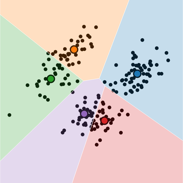
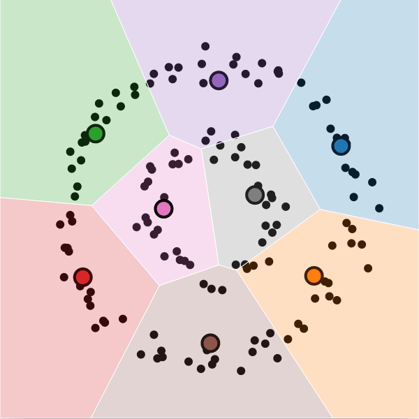
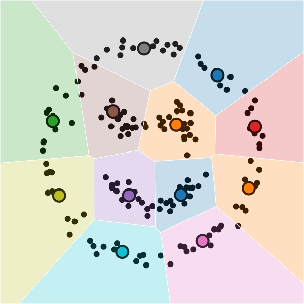
K-means is a centroid model -each cluster is represented by a central point. “K” represents the number of clusters, and “mean” is the aggregation operation applied to elements of a cluster to define the central location. Central points are called centroids or prototypes of the clusters.
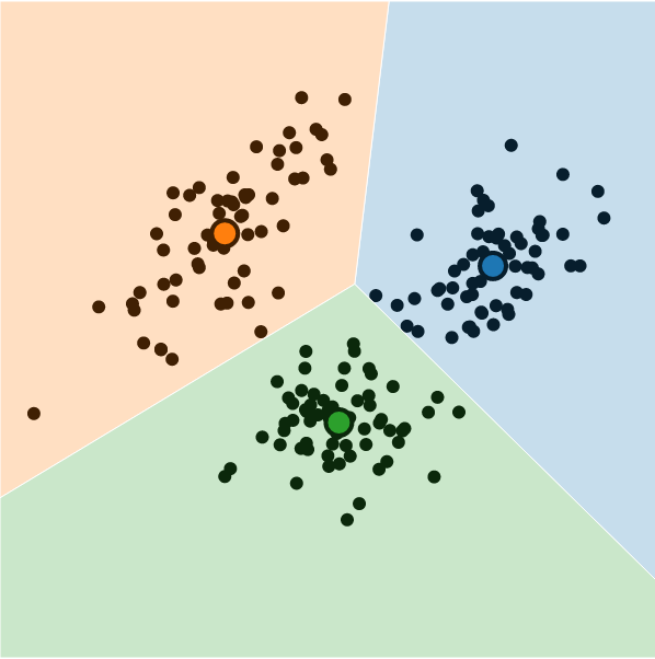
Black dots represent data points, coloured dots are centroids,
and coloured areas show cluster expansions.
The K-Means Algorithm
From a theoretical perspective, finding the optimal solution for a clustering problem is particularly difficult (NP-hard). Thus, all algorithms are only approximations of the optimal solution. The k-means algorithm, sometimes referred to as the Lloyd algorithm after its author (Lloyd, 1982), is an iterative process that refines the solution until it converges to a local optimum.
Let’s use some mathematical notations to formalize this:
- \( X = \{ \textbf{x}_1, \, \ldots ,\; \textbf{x}_n ;\, \textbf{x}_j \in \mathbb{R}^d \} \) denotes the set of data points of dimensions \( d \).
- \( C = \{ \textbf{c}_1, \, \ldots ,\; \textbf{c}_k ;\, \textbf{c}_i \in \mathbb{R}^d \} \) is the set of centroids.
- \( S = \{ S_1, \, \ldots ,\, S_k \} \) represents the groupings where \( S_i \) is the set of data points contained in the cluster \( i \). The number of samples in \( S_i \) is noted \( n_i \).
Notations can have superscripts to illustrate the iterative aspect of the algorithm. For example, \( C^t = \{ \textbf{c}^t_1,\, … ,\, \textbf{c}^t_k \} \) defines the centroids at step \( t \).
Given some data points and the number of clusters, the goal is to find the optimal centroids —those which minimize the within-cluster distance— also called the within-cluster sum squared error (SSE):
\[ C_{best} = \underset{C}{\arg\min} \sum_{i=1}^{k} \sum_{\textbf{x} \in S_i} \lVert \textbf{x} - \textbf{c}_i \rVert^2 \]
The training procedure is as follows:
-
Initialization: Often, there is no good prior knowledge about the location of the centroids. An effortless way to start is to define the centroids by randomly selecting \( k \) data points from the dataset (Forgy method).
In mathematical notation, we define \( C^0 \), the initial set of centroids, as a subset of data points with a cardinality of \( k \): \( C^0 \subset X \) with \( \vert C^0 \vert = k \). -
Assignment: For each data point, the distance to all centroids is computed. The data points belong to the cluster represented by the closest centroid. This is called a hard assignment because the data point belongs to one and only one cluster.
Data points are assigned to partitions as follows: \[ S^t_i = \{\textbf{x} \in X ;\; \lVert \textbf{x} - \textbf{c}_i \rVert < \lVert \textbf{x} - \textbf{c}_j \rVert, \; \forall 1 \leq j \leq k \} \] -
Update: Given all the points assigned to a cluster, the mean position is computed and defines the new location of the centroid. All centroids are updated simultaneously. \[ \forall 1\le i \le k, \,\, \textbf{c}^{t+1}_i = \frac{1}{\vert S^t_i \vert } \sum_{\textbf{x} \in S^t_i}{\textbf{x}} \]
-
Repeat steps 2 and 3 until convergence. The algorithm can stop after a predefined number of iterations. Another convergence criterion could be to stop whenever the centroids move less than a certain threshold during step 3.
Once the algorithm has converged and is used on new data, only the assignment step is performed.
Visualization
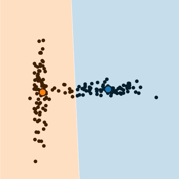
It is possible to visualize the decision boundaries.
To do so, we can generalize the definitions of the groups and include all possible elements rather than
only observed data points:
\[ S_i = \{\textbf{x} \in \mathbb{R}^d ;\; ||\textbf{x} - \textbf{c}_i || < || \textbf{x} - \textbf{c}_j ||, \; \forall 1 \le j \le k \} \]
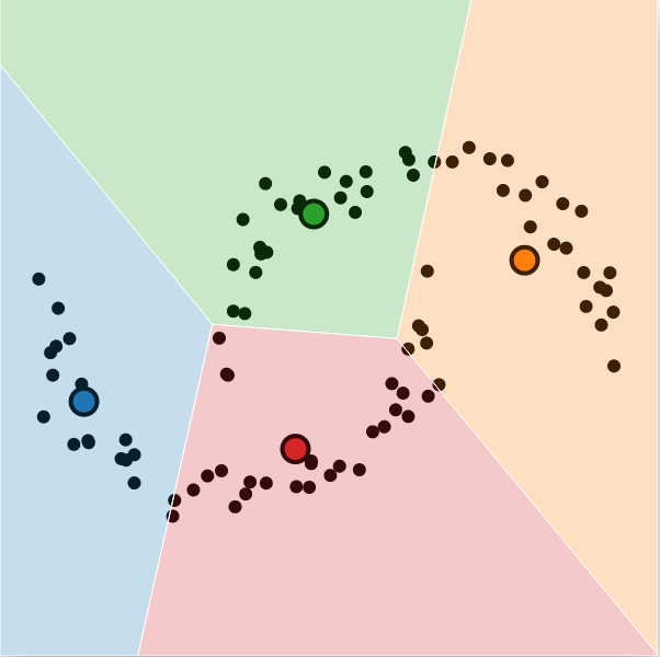
These are called Voronoi cells, and they look like this:
Python Implementation using Numpy
Although the algorithm could be implemented with plenty of nested for loops, it can execute several orders of magnitude faster if we leverage matrix arithmetic. Numpy (Harris et al., 2020) is an open-source Python library designed to ease the manipulation of vectors, matrices and arrays of any dimension. The core operations are written in C, a low-level language, to achieve fast runtime.
You can use conda or pip package managers to install Numpy.
conda: conda install numpy
pip: pip install numpy
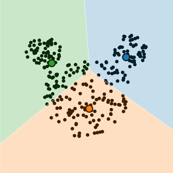
Let’s start by importing Numpy and creating some synthetic data generated from three normal distributions.
import numpy as np

blob1 = np.random.multivariate_normal(mean=[-3, 3], cov=[[3, 2], [2, 3]], size=100)
blob2 = np.random.multivariate_normal(mean=[5, 2], cov=[[2, 1], [1, 2]], size=100)
blob3 = np.random.multivariate_normal(mean=[0, -3], cov=[[2, 0], [0, 2]], size=100)
data = np.vstack([blob1, blob2, blob3])
The next step is to define a function for each step of the algorithm.
def pick_centroids(data, k):
    indexes = np.random.choice(len(data), size=k, replace=False)
    centroids = data[indexes]
    return centroids

def assign_cluster(data, centroids):
    # Pairwise squared L2 distances. Shape [n, k]
    distances = ((data[:, np.newaxis] - centroids)**2).sum(axis=2)
    # find closest centroid index. Shape [n]
    clusters = np.argmin(distances, axis=1)
    return clusters

def update_centroids(data, clusters, k):
    # Mean positions of data within clusters
    centroids = [np.mean(data[clusters == i], axis=0) for i in range(k)]
    return np.array(centroids)
The final step is to glue everything together inside a class:
class KMeans:
    def __init__(self, k=3):
        self.k = k

    def fit(self, data, steps=20):
        self.centroids = pick_centroids(data, self.k)
        for step in range(steps):
            clusters = assign_cluster(data, self.centroids)
            self.centroids = update_centroids(data, clusters, self.k)

    def predict(self, data):
        return assign_cluster(data, self.centroids)
Finally, we can instantiate an object, train it, and do the predictions.
kmeans = KMeans(k=3)
kmeans.fit(data)
clusters = kmeans.predict(data)
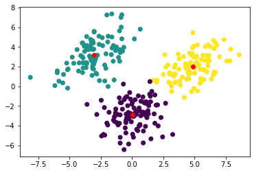
If you have Matplotlib installed (pip install matplotlib), you can visualize the data and the result.
import matplotlib.pyplot as plt
# Plot data points with cluster id as color
plt.scatter(data[:, 0], data[:, 1], c=clusters)
# Plot centroids
plt.scatter(kmeans.centroids[:, 0], kmeans.centroids[:, 1], c="red")
plt.show()
You should have something looking like this:
Go ahead and run the code step by step to build a better grasp of Numpy. Read the Numpy documentation about broadcasting operations to understand how the pairwise distance is computed with a single line of code.
I suggest you don’t use this code if it’s not for educational purposes. Scikit-learn (Pedregosa et al., 2011) is a very popular open-source Python library, built on top of Numpy, which implements the naive k-means algorithm, its variants, and many more machine learning algorithms.
Limitations and Variants
The strength of K-means is its conceptual simplicity. The logic —but also the implementation— is intuitive and straightforward. However, it is necessary to understand that the algorithm was built around restrictive hypotheses about the data distribution. Some tweaks and variants overcome some limitations.
Sensitivity to Initialization
The first drawback of k-means, which can easily be observed after a few runs, is the sensitivity of the algorithm to the initial locations of the centroids. Each possible initialization corresponds to a certain convergence speed and a final solution. Some solutions correspond to local minima and are far from optimal.
A naive way to address this sensitivity to initialization is to run the algorithm several times and keep the best model. Another solution to get around it is to use expert knowledge to hand-craft what could be a good initialization. A third solution is to come up with some heuristics to define a good initialization state. These rules are called seeding techniques.
Seeding techniques
Many seeding heuristics have been developed over time. K-means++ (Arthur & Vassilvitskii, 2006) is one of the most popular and the default initialization method in Scikit-learn (and Matlab). The motivation behind it is that spreading out the initial centroids is beneficial. Indeed, picking up spread centroids increases the chances that they belong in different clusters.
The k-means++ seeding algorithm is as follows:
- Randomly select the first set of centroids among the data points.
- For all data points, compute the distance to the closest centroid \( D(\textbf{x}) \).
- Pick up another centroid from the set of data points, given the weighted distribution proportional to the squared distances: \( p(\textbf{x}_i)= \frac{ D(\textbf{x}_i)^2 }{ \sum_{\textbf{x} \in X} D(\textbf{x})^2 } \)
- Repeat the two previous steps \( k-1 \) times.
The benefits in terms of convergence speed and final error outweigh the computational overhead for this initialization procedure; see the original paper (Arthur & Vassilvitskii, 2006) for details. If you are looking for a thorough comparison of seeding techniques, I recommend this recent review (Fränti & Sieranoja, 2019).
Keep in mind that a good initialization of the centroids should be as close as possible to the optimal solution. Thus, finding a good initialization is not easier than solving the clustering problem itself.
Harmonic Means
The authors of k-harmonic means (Zhang et al., 1999) claim their approach is significantly less sensitive to initialization. This algorithm does not optimize the SSE, but a different performance metric, which relies on a soft assignment and takes the sum over all data points of the harmonic average of the squared distance to all centroids. \[ C_{best} = \underset{C}{\arg\min} \sum_{\textbf{x} \in X} \frac{1}{ \sum_{i=1}^K \frac{1}{\lVert \textbf{x} - \textbf{c}_i \rVert^2} } \]
Looking for the minimum of this expression with respect to centroids leads to a different update rule:
\[
\begin{aligned}
\forall 1\le i \le k, \,\, \textbf{c}^{t+1}_i &= \sum_{\textbf{x} \in X} \frac{\alpha_{i,\textbf{x}}^t \textbf{x}}{\alpha_{i,\textbf{x}}^t} \\
\text{with}\;\, \alpha_{i,\textbf{x}}^t &= \frac{1}{\vert\vert \textbf{x} - \textbf{c}_i^t \vert\vert^3 \left( \sum_{j=1}^K \frac{1}{\vert\vert \textbf{x} - \textbf{c}_j^t \vert \vert^2 } \right)^2 }
\end{aligned}
\]
Check out the paper if you would like to implement k-harmonic means. They propose an efficient algorithm that reduces numerical instabilities.
Computational Time Complexity
The assignment step time complexity is \( O(nkd) \) where \( n \) is the number of samples, \( k \) is the number of clusters, and \( d \) is the input space dimension. This complexity is the consequence of computing the pair-wise distance between all data points and all centroids. The update step has a time complexity of \( O(nd) \). The mean is computed along \( d \) dimensions for \( k \) clusters, each containing an average of \( n/k \) data points.
The overall time complexity at each step of the Lloyd algorithm is therefore \( O(nkd) \). If all these values increase two-fold at once, then the algorithm will be eight times slower—not ideal. In addition, the number of necessary iterations to reach convergence grows sublinearly with \(k\), \(n\) and \(d\).
Dimensionality Reduction
There are some ways to mitigate this scaling problem. The first one is to retain only the relevant dimensions with a feature selection. The second is to project the data points into a smaller space with principal components analysis (PCA), independent component analysis (ICA), or linear discriminant analysis (LDA).
Batch Processing
A second approach to reducing the computational complexity is to use fewer samples at each iteration. Rather than working with all data points, the algorithm only manipulates a randomly selected subset. This variant is called mini-batch k-means. We usually want the batch size, noted \( b \), to be far greater than the number of clusters and much lower than the number of samples (\( k \ll b \ll n \)).
Triangular Inequality
We know the shortest path between two points is to follow a straight line rather than to stop somewhere else in between. In mathematics this is known as the triangular inequality: \[ \forall \textbf{x}, \textbf{y}, \textbf{z} \in \mathbb{R}^d ,\;\, \vert\vert \textbf{x} - \textbf{z} \vert\vert \leq \vert\vert \textbf{x} - \textbf{y} \vert\vert + \vert\vert \textbf{y} - \textbf{z} \vert\vert \]
We can leverage this for our case: given a data point \( \textbf{x} \) and two centroids \( \textbf{c}_1 \) and \( \textbf{c}_2 \), if \( \vert\vert \textbf{x} - \textbf{c}_1 \vert\vert \leq \frac{1}{2} \vert\vert \textbf{c}_1 - \textbf{c}_2 \vert\vert \) then \( \vert\vert \textbf{x} - \textbf{c}_1\vert\vert \leq \vert\vert \textbf{x} - \textbf{c}_2 \vert\vert \), which means \( \textbf{x} \) belongs to the cluster represented by \(\textbf{c}_1\). Consequently, we do not not need to compute \( \vert\vert \textbf{x} - \textbf{c}_2 \vert\vert \).
Over the course of the training, the Elkan algorithm (Elkan, 2003) keeps track of the upper bounds for the distances between all data points and the centroids (noted \( u_{\textbf{x},\textbf{c}} \) ). Suppose \( u_{\textbf{x},\textbf{c}_1} \geq \vert\vert \textbf{x} - \textbf{c}_1 \vert\vert \), then we can spare the computations of \( \vert\vert \textbf{x} - \textbf{c}_2 \vert\vert \) if \( u_{\textbf{x},\textbf{c}_1} > \vert\vert \textbf{c}_1 - \textbf{c}_2 \vert\vert \). The upper bounds get updated at each iteration as the centroids keep on moving.
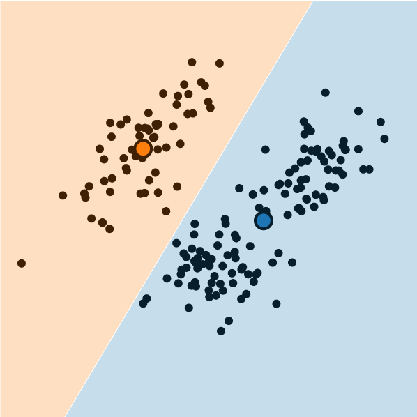
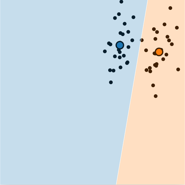
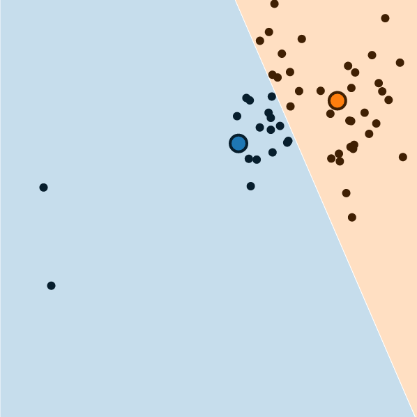
Sensitivity to Outliers
The centroid locations are defined as the mean positions of the data points within each cluster. However, the mean is an estimator sensitive to outliers. Outliers are data points that are significantly different from the other ones (out of distribution samples). Fig.3 illustrates this issue, where two data points out of distribution have a disproportionate impact on the final result. Not only are some points not assigned to the right cluster, but the decision boundary is ultimately different.
If possible, a solution could be to preprocess the data by filtering out the outliers. A different remedy could be to weight each data point. During the update step, weighted-mean is therefore used. Weighted k-means can reduce the impact of the outliers and avoid the need for a hard decision in the preprocessing. Finding a good weighting strategy is not easy and might take a few trials.
Different Aggregators
There are two more variants of k-means designed to reduce the influence of outliers. For the first one, the centroids are no longer defined as the mean locations but as the median positions. The algorithm is rightfully called k-medians. K-means minimize the within cluster-variance (L2-norm) while k-medians minimize the absolute deviation (L1-norm). For k-medians, the update rule becomes:
\[ \forall 1\le i \le k, \,\, c^{t+1}_i = \text{median}( S^t_i ) \]
The second adaptation enforces some restrictions to centroids. Rather than taking any possible locations, the centroids are restricted to the set of data points. This algorithm is called k-medoids (or Partitioning Around Medoids). A medoid is the most central representant in a cluster which minimizes the sum of distances to other data points. This distance metric makes k-medoids more robust to outliers. For k-medoids, the optimal solution is given by:
\[ C_{best} = \underset{X}{\arg\min} \sum_{i=1}^{k} \sum_{\textbf{x} \in S_i} \lVert \textbf{x} - \textbf{c}_i \rVert \]
Finding the right medoids requires a different algorithm (out of scope for this post) and has a higher computational complexity of \( O(k(n-k)^2) \) at each iteration step. See PAM, CLARA, and CLARANS algorithms (Schubert & Rousseeuw, 2019) if you are interested.
Shape and Extent of Clusters
Convexity of Partitions
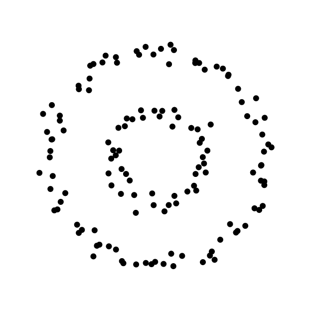
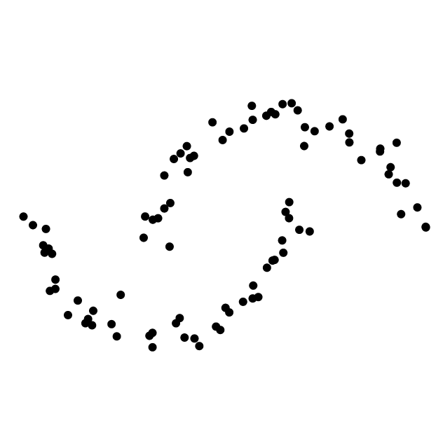
K-means, and all its variants, minimize distortion and optimize the clusters for compactness. The implicit assumption is that clusters are roughly spherical (isotropic, uniform in all directions). Depending on the distribution of data points, some clusters might not be exactly spherical, but they will at least form convex partitions. Convex means that for any two points in the same cluster, the whole segment from one point to the other is fully contained inside the Voronoi cell.
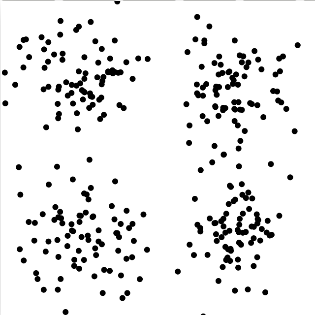
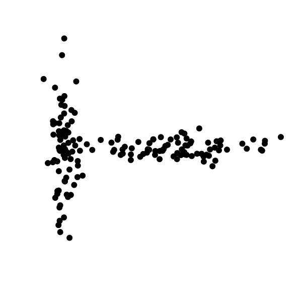
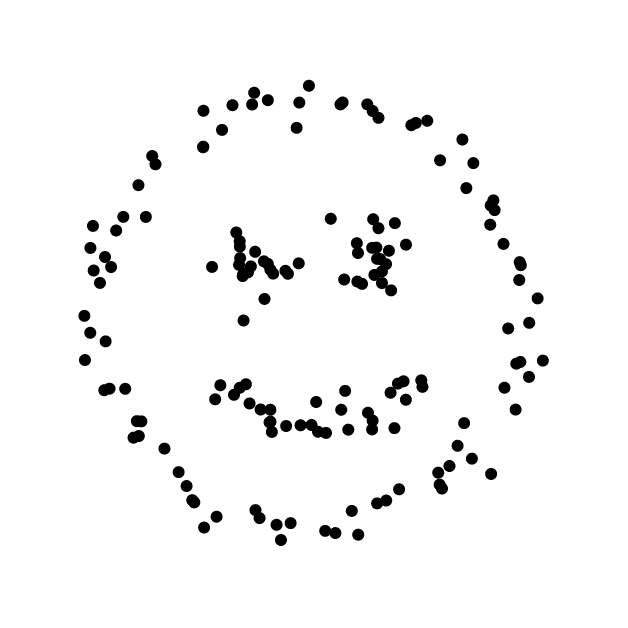
Some good examples of failing cases are concentric circles, half-moons, and the smiley, as illustrated in the figure below. There is no way for k-means to isolate the inner ring from the external ring, as the outermost partition will not be convex. The same problem applies to the 4 components of the smiley. For the two half-moons, the geometrical properties of each cluster cannot be captured.
One partial solution is to overestimate the number of clusters and merge the partitions later on. However, that might not be easy for high-dimensional data, and it will never really compensate if the data distribution violates the initial assumption of spherical/convex clusters.
One might want to use the kernel trick to operate in a higher dimensional space. The hope is that in the projected space the data will comply with the spherical distribution hypothesis. Finding the right kernel function could be cumbersome.
Similar Expansions
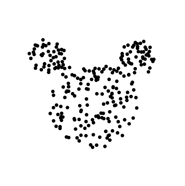
A further limitation is the relative size of clusters. By placing the decision boundaries halfway between centroids, the underlying assumption is that clusters are evenly sized along that direction. The size is defined as the spatial extent (area, volume, or Lebesgue measure) —not the number of data points assigned inside the cluster.
Once again, some datasets with complex geometrical shapes might not match this assumption. The perfect example is the Mickey Mouse dataset.
Finally, the k-means could fail if data arises from blobs with similar sizes, but some generate far fewer observations. This is somewhat related to the initialization problem: selecting a centroid from the underrepresented class is less likely.
To sum up, k-means clustering assumes the clusters have convex shapes (e.g. a circle, a sphere), all partitions should have similar sizes, and the clusters are balanced.
Capturing Variances
K-means and its variants only learn the central location of clusters—nothing more. It would be relevant to also capture the spatial extent of each cluster. The Gaussian Mixture Model (GMM) was designed to capture the mean location and standard deviation of the data.
GMM computes the probability for all data points to belong to a cluster, for all clusters. This is called a soft assignment, in opposition to the hard assignment to one and only one cluster used by k-means. GMM is a powerful tool. There is a lot to say about it, but that will be a story for another time.
Optimal Number of Clusters
Last but not least, finding the optimal number of clusters is necessary to achieve good performance. Priors or domain knowledge can be very handy for this task. To this day, more than 30 methods have been published on this topic. I will try to cover the most common methods.
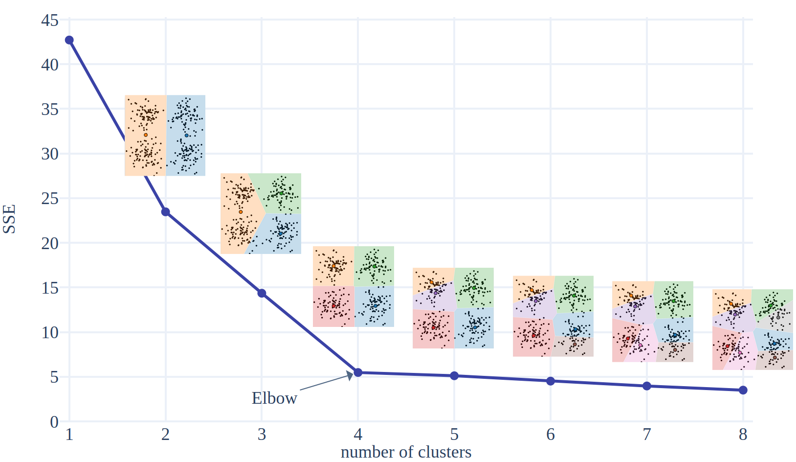
The Elbow Method
First of all, we need to define a metric which tells how compact the clusters are. A pertinent metric for this is the within-cluster sum squared error (\(SSE\) or \(WSS\)). It is defined as the sum of squared distance between each point and its closest centroid.
\[ SSE(k) = \sum_{i=1}^{k} \sum_{\textbf{x} \in S_i} \vert\vert \textbf{x} - \textbf{c}_i \vert\vert^2 \]
This function is strictly decreasing when applied on converged models. At first, when we add clusters it gets easier to model the data. But after a certain point, increasing the number of clusters brings little additional benefits, as it only splits clusters into sub-groups or starts modelling the noise. The Elbow method (Thorndike, 1953) is a heuristic to find this point of diminishing return. The analysis is performed by plotting the evolution of the explained variance as the number of clusters grows. The optimal number of clusters is located at the bend, the elbow of the curve.
\( SSE \) is often applied once the model has converged. However, it can also be used as a stopping criteria for the algorithm. If \( SSE \) is computed at the end of each iteration, a heuristic could be to stop the training when the \( SSE \) decreases less than a certain threshold compared to the previous step.
Gap Statistic
The Elbow Method is far from ideal. The elbow is not formally defined, and a visual inspection is necessary to localise it. Consequently, the estimation of the optimal number of clusters can be subjective. Not all SSE curves will have a sharp elbow like in the example above!
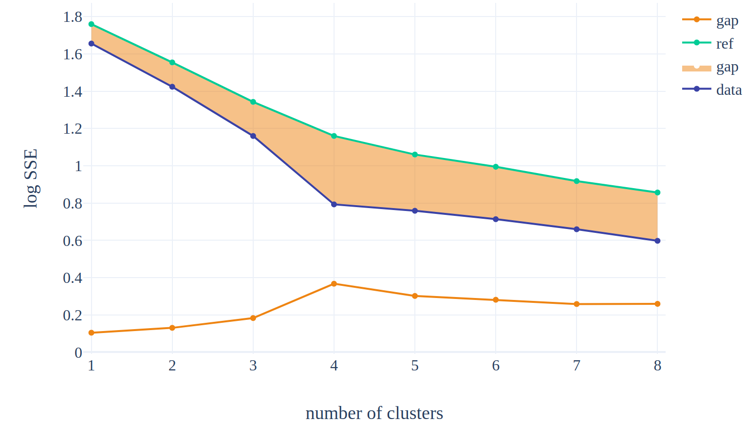
The gap statistic analysis (Tibshirani et al., 2001) addresses this problem. The idea behind it is to compare the SSE measured on the data with the SSE computed on a dataset without obvious clustering (data with a null reference distribution). The SSE on the data should be further away from the reference value for the optimal number of clusters.
The equation looks like this :
\[ G(k) = \log SSE(X^*, k) - \log SSE(X, k) \]
We denote by \( X^* \) a dataset with data points uniformly distributed in the interval defined by the minimum and maximum values of \( X\) along each \( d \) component.
The expected SSE on the null distribution, the first term of the equation, is estimated with bootstrapping. This means we sample \( B \) different datasets \(X_b^* \; \forall 1 \leq b \leq B\) and compute the mean logarithm of SSE. The estimation gets more accurate with higher values of B. However, keep in mind that \( G_B(k) \) is only computed once k-means has converged \( B+1 \) times. The expression of the gap function becomes:
\[ G_B(k) = \frac{1}{B} \sum_{b=1}^{B} \log SSE(X_b^*, k) - \log SSE(X, k) \]
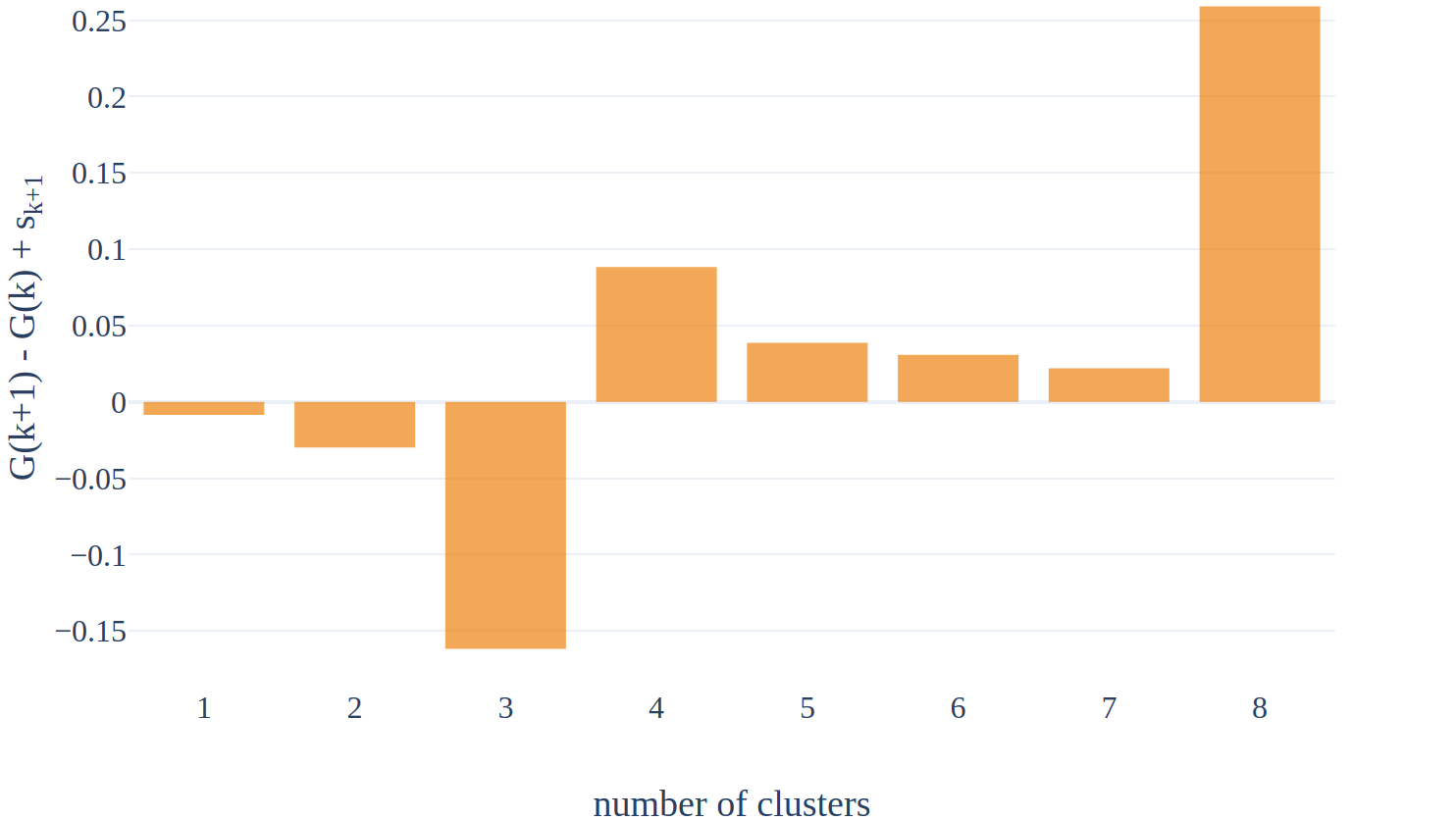
The optimal number of clusters is the smallest k such that \( G(k) \geq G(k+1) - s_{k+1} \) where \( s_k = \sqrt{1 + 1/B}\;\text{std}_B(\log SSE(X_b^*, k)) \) accounts for the simulation error.
Our toy example is simple enough so identifying the k which meets this condition is straightforward (k=4).
Silhouette Analysis
Silhouette coefficient (Rousseeuw, 1987) is a quality measurement for partitioning. The silhouette score measures how close a data point is to its counterparts in the same cluster compared to other elements in other clusters. The score captures the cohesion (within-cluster distances) and the separation (inter-cluster distances).
The average dissimilarity of a data point \( \textbf{x} \) with elements in a cluster is defined as:
\[ d(\textbf{x}, S_i) = \frac{1}{n_i - 1} \sum_{\textbf{x}_i \in S_i} \vert\vert \textbf{x}_i - \textbf{x} \vert\vert \]
The cohesion score (the lower, the better) of \( \textbf{x} \), which belongs to partition \( S_{\textbf{x}} \), is the intra-cluster distance: \( a(\textbf{x}) = d(\textbf{x}, S_{\textbf{x}}) \). The partition that does not contain \( \textbf{x} \) and minimize \( d(\textbf{x}, S_i) \) is called the neighboring cluster. The separation score (the higher, the better) is defined as the average dissimilarity of \( \textbf{x} \) with the neighbouring cluster: \( b(\textbf{x}) = \min_{i, \textbf{x}\notin S_i} d(\textbf{x}, S_i) \). The silhouette coefficient combines these two scores:
\[ s(\textbf{x}) = \frac{b(\textbf{x}) - a(\textbf{x})}{\max\{a(\textbf{x}), b(\textbf{x})\}} \]
If the cluster only contains 1 data point, the silhouette score is set to 0. The score varies from -1 to 1. A score close to 1 represents data points well assigned to clusters. If the score is positive, the data point is on average closer to elements in the cluster it belongs to rather than elements in the neighbouring cluster. On the contrary, if it is negative, the data point should belong to the neighbouring cluster.
The mean silhouette score over all data points is a measure of the partitioning quality. This quality score can be computed for several values of \(k\). The best number of clusters yields the highest average silhouette coefficient.
It is possible to gain much more insight about the quality of partitioning by plotting the sorted silhouette coefficients per cluster for different numbers of clusters. The silhouette analysis looks like this:
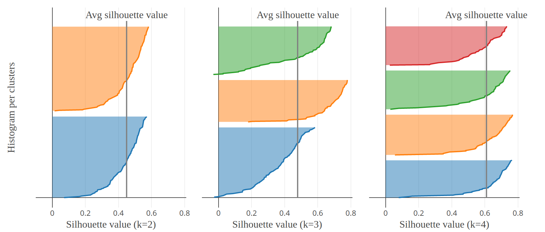
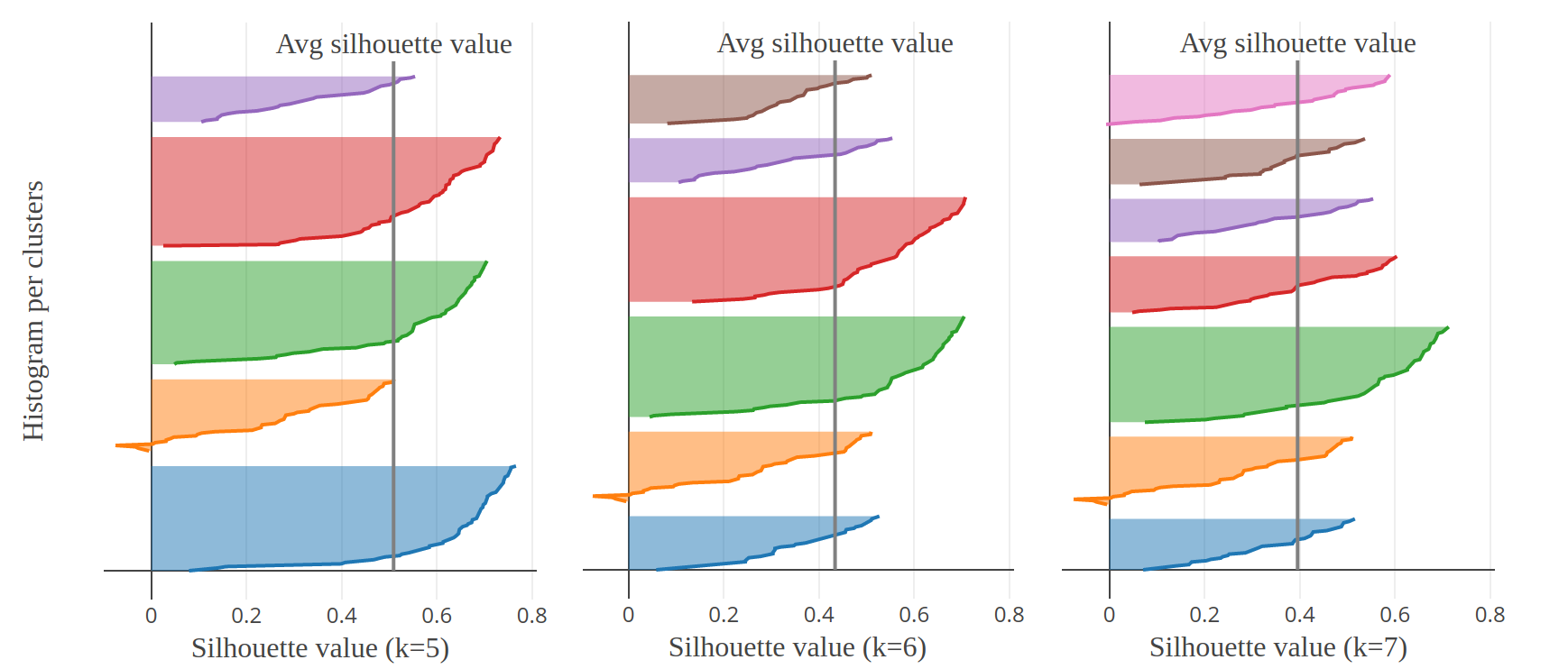
For the optimal number of clusters, the silhouette plots should:
- have the same thickness (same number of observations)
- have the same profile
- intersect with the average silhouette score
In Fig.8, we can rule out \(k=3,5,6,7\). The graphical analysis is ambivalent between \(k=2\) and \(k=4\). However, the latter has a higher average value. The conclusion of the analysis is that best results are obtained with \(k=4\).
The Elbow method has a linear time complexity of \(O(nd)\). The silhouette computes all pairwise distances, so time complexity jumps to \(O(n^2d)\). It’s not cheap, and in fact it’s worse than the Lloyd algorithm itself on most datasets.
Measures of Information
A good estimator of the model performance should take into account the quality of the model but should also penalise for the complexity of the model. Bayesian Information Criterion (BIC) (Schwarz & others, 1978) and Akaike Information Criterion (AIC) (Akaike, 1974) measure the statistical quality of a model and respect this parsimony principle (more parameters should not be added without necessity). For both metrics, the lower the better.
For k-means, the simplest expressions for \( BIC \) and \( AIC \) are defined as: \begin{aligned} BIC &= \frac{SSE}{\hat\sigma^2} + kd\log(n) \\ AIC &= \frac{SSE}{\hat\sigma^2} + 2kd \end{aligned}
\( \hat\sigma^2 \) is the average intra-cluster variance defined on a model with a very high number of clusters (Friedman et al., 2001, sec. 7.7): \( \hat\sigma^2 = \frac{SSE(k’)}{k’},\; k’>k \). It is worth computing \( \hat\sigma^2 \) for several values of \( k’ \). Small \( k’ \) penalizes models with high number of clusters more heavily
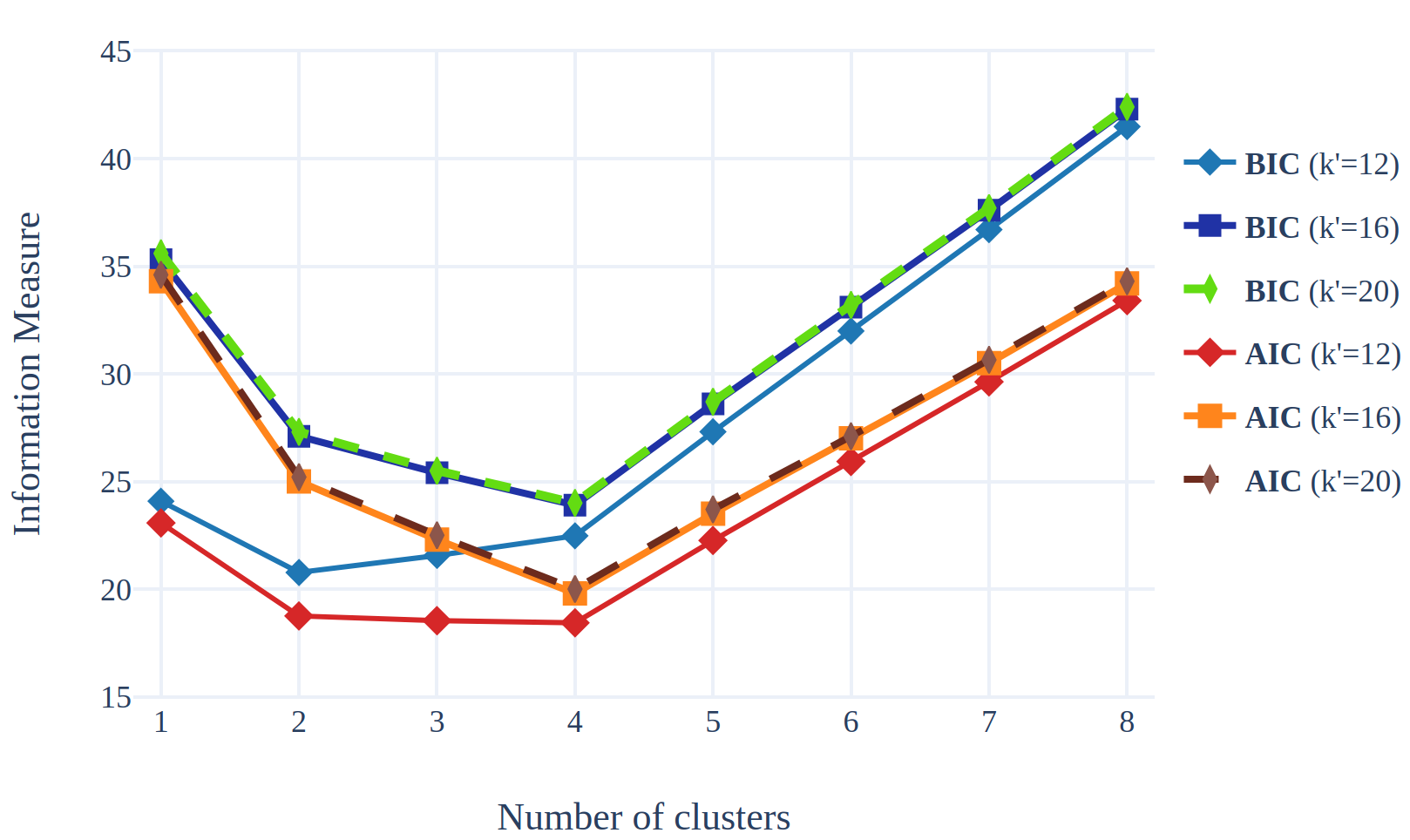
From the above figure, we can see that curves for \(k’=16\) and \(k’=20\) are overlapping, for both \( BIC \) and \(AIC\) since the average intra-cluster variances are nearly equal. In both cases, and for both metrics, the optimal number of clusters is 4.
The story and the conclusion is a bit different for \( k’=12 \). The minimum for \( BIC \) is reached for \( k = 2 \) but the minimum for \( AIC \) is obtained with \( k = 4 \). This illustrates that small \(k’\) leads to models with fewer clusters. It also shows that BIC yields a higher penalty than \(AIC\).
This is not the whole story. Click to expand if you like equations!
\(BIC\) and \(AIC\) are originally defined as:
\( BIC = p\log(n) - 2 \log\left(L (M; X) \right) \) and \( AIC = 2p - 2 \log\left(L (M; X) \right) \)
where \( M \) is the model, \( p \) is the number of free-parameters of \( M \),
and \( L (M; X) \) is the model likelihood.
With k-means, we can heavily rely on the assumption that data arises from identical isotropic blobs. Observed data points can be decomposed as \( \textbf{x} = \mu + e, \; \forall \textbf{x} \in X \) where the \( \mu \) is one of the centroids, \(\mu \in C \); and the error follows a multivariate Gaussians, \( e \sim \mathcal{N}(0,\,\sigma^{2}I_d)\).
Given a partition of the space, the probability to observe a data point \( \textbf{x} \) is therefore defined by: \[ P(\textbf{x} \vert S) = \frac{n_i}{n} \frac{1}{\sqrt{2 \pi \sigma^2}^{d}} \exp \left( -\frac{\vert \vert \textbf{x} - \textbf{c}_i \vert \vert_2^2}{2\sigma^2} \right) \]
This can be injected into the log-likelihood: \[ \begin{aligned} \log & L(S; X) = \log \prod_{\textbf{x} \in X} P(\textbf{x} \vert S) = \sum_{i=1}^{k} \sum_{\textbf{x} \in S_i} \log P(\textbf{x} \vert S) \\ &= \sum_{i=1}^{k} \left[ n_i \log\left(\frac{n_i}{n}\right) - \frac{\sum_{\textbf{x} \in S_i} \vert \vert \textbf{x} - \textbf{c}_i \vert \vert_2^2}{2\sigma^2}\right] - \frac{nd}{2}\log(2\pi\sigma^2) \end{aligned} \] If we consider that all clusters are evenly balanced, and if we assume \( \sigma^2 \) to be fixed, then \( BIC \) and \(AIC\) are equal to the previous equation with an additive constant. Even if \( \sigma^2 \) is considered fixed, it is unknown. Its value is estimated in a low-bias regime.
Now, let's assume \( \sigma^2 \) can be estimated from the data. The unbiased estimator of the variance for each cluster gives: \[ \forall 1\le i \le k, \; \hat\sigma_i^2 = \frac{1}{d(n_i - 1)} \sum_{\textbf{x} \in S_i} \vert\vert \textbf{x} - \textbf{c}_i \vert\vert^2 \] Combined with the definition of SSE, we end up with: \[ SSE = \sum_{i=1}^{k} \sum_{\textbf{x} \in S_i} \vert\vert \textbf{x} - \textbf{c}_i \vert\vert^2 = \sum_{i=1}^k d(n_i - 1) \hat \sigma_i^2 \]
With the underlying assumption that all clusters have the same extent, we have \( \hat\sigma^2 = \hat \sigma_i^2 \). In conclusion, the unbiased estimation of the variance is: \[ \hat\sigma^2 = \frac{1}{d(n-k)} \sum_{i=1}^{k} \sum_{\textbf{x} \in S_i} \vert\vert \textbf{x} - \textbf{c}_i \vert\vert^2 = \frac{SSE}{d(n-k)} \]
Going back to the log-likelihood formula, it can be simplified into: \[ \begin{aligned} \log & L(S; X) = \sum_{i=1}^{k} \left[ n_i \log\left(\frac{n_i}{n}\right) \right] - \frac{d(n-k)}{2} - \frac{nd}{2}\log(2\pi\sigma^2) \end{aligned} \] In the end, knowing that there are \( p=k\times d \) free parameters for k-means, the \( BIC \) and \( AIC \) expressions become: \[ \begin{aligned} BIC & =(2n + dk)\log(n) + d(n-k) + nd\log(2\pi\sigma^2) - 2 \sum_{i=1}^{k} n_i \log\left(n_i\right) \\ AIC & = 2n\log(n) + d(n+k) + nd\log(2\pi\sigma^2) - 2 \sum_{i=1}^{k} n_i \log\left(n_i\right) \\ \text{with}&\; \sigma^2 = \frac{SSE}{d(n-k)} \end{aligned} \] There is still one limitation with these equations: they consider the assignment as the true label for classification rather than taking into account the uncertainty in this assignment. I recommend this article (Hofmeyr, 2020) which shows that the number of free parameters is underestimated.Conclusion
K-means’ high notoriety is certainly due to its simplicity and ease of implementation. However, it has quite a few limitations: the dependence on the initial centroids, the sensitivity to outliers, the spherical/convex clusters, and the troubles of clustering groups of different density and spatial extent.
It is also necessary to standardize the data to have zero mean and unit standard deviation. Otherwise, the algorithm might struggle or give too much importance to certain features.
Interview Questions
Try to answer the following questions to assess your understanding of k-means and its variants. These questions are often asked during interviews for data science positions.
- What is clustering?
- Is clustering a supervised or an unsupervised technique?
- Can you describe the K-means algorithm?
- What is its complexity? How would you reduce the number of computations?
- What are some termination criteria?
- What is the difference between hard and soft assignments?
- What are some weaknesses of k-means?
- The algorithm has some assumptions about the data distribution. What are they?
- How do you find the optimal number of clusters?
- How come two different executions of the algorithm produce different results? How does one address this problem?
- What kind of preprocessing would you apply to the data before running the algorithm?
- Is the algorithm sensitive to outliers? If yes, how could you mitigate the problem?
- What are the applications of k-means clustering?
References
- Lloyd, S. (1982). Least squares quantization in PCM. IEEE Transactions on Information Theory, 28(2), 129–137.
- Harris, C. R., Millman, K. J., van der Walt, S. J., Gommers, R., Virtanen, P., Cournapeau, D., Wieser, E., Taylor, J., Berg, S., Smith, N. J., & others. (2020). Array programming with NumPy. Nature, 585(7825), 357–362.
- Pedregosa, F., Varoquaux, G., Gramfort, A., Michel, V., Thirion, B., Grisel, O., Blondel, M., Prettenhofer, P., Weiss, R., Dubourg, V., Vanderplas, J., Passos, A., Cournapeau, D., Brucher, M., Perrot, M., & Duchesnay, E. (2011). Scikit-learn: Machine Learning in Python. Journal of Machine Learning Research, 12, 2825–2830.
- Arthur, D., & Vassilvitskii, S. (2006). k-means++: The advantages of careful seeding. Stanford.
- Fränti, P., & Sieranoja, S. (2019). How much can k-means be improved by using better initialization and repeats? Pattern Recognition, 93, 95–112.
- Zhang, B., Hsu, M., & Dayal, U. (1999). K-harmonic means-a data clustering algorithm. Hewlett-Packard Labs Technical Report HPL-1999-124, 55.
- Elkan, C. (2003). Using the triangle inequality to accelerate k-means. Proceedings of the 20th International Conference on Machine Learning (ICML-03), 147–153.
- Schubert, E., & Rousseeuw, P. J. (2019). Faster k-medoids clustering: improving the PAM, CLARA, and CLARANS algorithms. International Conference on Similarity Search and Applications, 171–187.
- Thorndike, R. L. (1953). Who belongs in the family? Psychometrika, 18(4), 267–276.
- Tibshirani, R., Walther, G., & Hastie, T. (2001). Estimating the number of clusters in a data set via the gap statistic. Journal of the Royal Statistical Society: Series B (Statistical Methodology), 63(2), 411–423.
- Rousseeuw, P. J. (1987). Silhouettes: a graphical aid to the interpretation and validation of cluster analysis. Journal of Computational and Applied Mathematics, 20, 53–65.
- Schwarz, G., & others. (1978). Estimating the dimension of a model. The Annals of Statistics, 6(2), 461–464.
- Akaike, H. (1974). A new look at the statistical model identification. IEEE Transactions on Automatic Control, 19(6), 716–723.
- Friedman, J., Hastie, T., & Tibshirani, R. (2001). The elements of statistical learning (Vol. 1, Number 10). Springer series in statistics New York.
- Hofmeyr, D. P. (2020). Degrees of Freedom and Model Selection for k-means Clustering.
- Schonlau, M. (2002). The clustergram: A graph for visualizing hierarchical and nonhierarchical cluster analyses. The Stata Journal, 2(4), 391–402.