Learning to Land on Mars with Reinforcement Learning
Once in a while, a friend who is either learning to code or tackling complex problems drags me back to CodinGame However, I tend to put one type of challenge aside: optimal control systems. This kind of problem often requires hand-crafting a good cost function and modeling the transition dynamics. But what if we could solve the challenge without coding a control policy? This is the story of how I landed a rover on Mars using reinforcement learning.
CodinGame Mars Lander
This game’s goal is to land the spacecraft while using as few propellants as possible. The mission is successful only if the rover reaches a flat ground, at a low speed, without any tilt.
For each environment, we’re given Mars’s surface as pairs of coordinates, as well as the lander’s current state. That state includes position, speed, angle, current engine thrust, and remaining fuel volume. At each iteration, the program has less than 100ms to output the desired rotation and thrust power.
One test case looks like this:
Coding the Game
The CodinGame platform is not designed to gather feedback on millions of simulations and improve on them. The only way to circumvent this limitation is by reimplementing the game.
The Interface
Because I wanted to do some reinforcement learning, I decided to follow the Gym package’s Environment class interface. Gym is a collection of test environments used to benchmark reinforcement learning algorithms. By complying with this interface, I could use many algorithms out of the box (or so I thought).
All Gym Environments follow the same interface, with two fields and three methods:
action_spaceobservation_spacereset(): called to generate a new gamestep(action): returns the new observations of the environment given a specific actionrender(): visualizes the agent in its environment
At first, I thought I could go without implementing render, but I was wrong.
As with any other machine learning task, visualization is of the utmost
importance for debugging.
Action Space
The algorithm controls the spacecraft’s thrust and orientation. The thrust has 5 levels between 0 and 4, and the angle is expressed in degrees between -90 and 90.
Rather than working in absolutes values, I decided that the action space would be a relative change in thrust and angle. The engine supports only a +/-1 change in thrust, and the orientation cannot change more than 15 degrees in absolute value.
Thrust and angle can be represented with categorical variables, with 3 and 31 mutually exclusive values respectively. Another possible characterization, which I decided to use, is to represent the action space as two continuous variables. For stability during the training, I normalized these values between -1 and 1.
Observation Space and Policy Network
Defining the observation space is a bit more challenging than it is for the action space. First, the agent expects a fixed-length input, but the ground is provided as a broken line with up to 30 points. To fulfill this requirement, I iteratively broke the longest segment into two by adding an intermediate point, until I reached thrity 2D points, for a total of 60 elements.
I then concatenated to these 60 elements the seven values that fully characterize the rover’s dynamic: x and y position, horizontal and vertical speed, angle, current thrust, and remaining propellant. I normalized these values between 0 and 1, or -1 and 1 if negative values are allowed.
In the early experiments, the fully connected policy was clearly struggling to identify the landing pad. The rover exhibited completely different behavior when the ground was translated horizontally because a slight offset creates a completely different representation of the ground once the surface is broken down into 30 points.
Changing the policy to a convolutional neural network (CNN) could have helped identify the landing area. By design, CNNs (unlike MLP) are translation equivariant. In addition, CNNs could have also eliminated the problem of fixed-length input I addressed above. Indeed, their number of parameters is independent of the input size.
After a few trials, it became clear that this approach would require a lot more effort to achive success. When using a CNN to extract an abstract ground representation, at some point these features need to be merged with the rover state. When should they merge? What should be the CNN’s capacity compared to that of the MLP? How should both networks be initialized? Would they work with the same learning rate? I ran a few experiments, but none of them were firmly conclusive.
In the end, to avoid going mad, I decided to use an MLP-based policy but to help the agent by providing a bit more information. The trick was to add the x and y coordinates of the two extremities of the flat section. This extra information can easily be computed by hand, so why not feed it to the model?
Simulation
When implementing the reset() function, I wanted to utilize as many
environments as possible. I initially thought that generating a random ground surface
and random rover state would do the job.
However, it turned out that not all these environments could be solved. For example, the rover might exit the frame before compensating for the initial speed, or the solution might consume an extremely high propellant volume. Finding a valid initial state might be as hard as solving the problem itself.
Clearly these unsolvable cases were penalising the training. This comes as no surprise; the same rule applies for any other machine learning task or algorithm. In the end, I decided to start from the five test cases CodinGame provided and to apply some random augmentations.
Reinforcement Learning
Policy Gradient
In reinforcement learning, an agent interacts with the environment via its actions at each time step. In return, the agent is granted a reward and is placed in a new state. The main assumption is that the future state depends only on the current state and the action taken. The objective is to maximise the rewards accumulated over the entire sequence.
Two classes of optimization algorithms are popular: Q-learning and policy gradient methods. The former aims to approximate the best transition function from one step to another. The latter directly optimizes for the best action. Despite being less popular, policy gradient methods have the advantage of supporting continuous action space and tend to converge faster.
For this task, I used a policy gradient method known as Proximal Policy Optimization (a.k.a PPO). In its revisited version, PPO introduces a simple twist to the vanilla policy gradient method by clipping the update magnitude. By reducing the variance and taking smaller optimization steps, the learning becomes more stable, with fewer parameter tweaks.
If you want to learn more about PPO and its siblings, I recommend the article Policy Gradient Algorithms by Lilian Weng, Applied AI Research Lead at OpenAI.
Action Noise
In the first experiments, the rover was very shaky, as its tilt oscillated around the optimal value. To eliminate this jerky motion, I used gSDE, which stands for generalized State-Dependent Exploration.
In reinforcement learning, it’s important to balance exploitation with exploration. Without exploring the action space, the agent has no way to find potential improvements. The exploration is often achieved by adding independent Gaussian noise to the action distribution.
The gSDE authors propose a state-dependent noise. That way, during one episode, the action remains the same for a given state rather than oscillating around a mean value. This exploration technique leads to smoother trajectories.
Reward Shaping
The reward is an incentive mechanism that tells the agent how well it’s performing. Crafting this function correctly is a big deal, given that the goal is to maximise the cumulative rewards.
Reward Sparsity
The first difficulty is reward sparsity. Let’s say we want to train a model to solve a Rubik’s cube. What would be a good reward function, knowing that there is only one good solution among 43,252,003,274,489,856,000 (~43 quintillion) possible states? It would take years to solve if we relied only on luck. If you’re interested in this problem, have a look at Solving the Rubik’s Cube Without Human Knowledge.
In our case, the rover has correctly landed if it grounds on a flat surface with a tilt angle of exactly 0° and a vertical and horizontal speed lower than 40 m/s and 20 m/s respectively. During training, I decided to loosen the angle restriction to anything between -15° and 15°, which increased the chances of reaching a valid terminal state. At inference, some post-processing code compensates for the rotation when the rover is about to land.
Reward Scale
If the rover runs out of fuel, or if it leaves the frame, it receives a negative reward of -150, and the episode ends. A valid terminal state yields a reward equal to the amount of remaining propellant.
By default, if the rover is still flying, it earns a reward of +1. In general, positive rewards encourage longer episodes, as the agent continues accumulating. On the other hand, negative rewards urge the agent to reach a terminal state as soon as possible to avoid penalties.
For this problem, shorter episodes should ideally consume less fuel. However, using the quantity of remaining fuel as a terminal reward creates a massive step function that encourages early misson completion. By maintaining a small positive reward at each step, the rover quickly learns to hover.
For the rest, not all mistakes are created equal. I decided to give a reward of -75 if speed and angle were correct when touching non-flat ground, as well as a -50 reward if the spacecraft crashed on the landing area. Without more experiments, it’s unclear whether if the distinction of collisions represents any advantage.
Not Taking Shortcuts
Previously, I talked about helping the model identify the arrival site. One idea was to change the policy structure by replacing the MLP with a CNN. I used the solution of adding this information in the input vector. A third possibility was to change the reward function to incorporate a notion of distance to the landing area.
I ran a few experiments in which the reward was the negative Euclidean distance between the landing site and the crash site. As it turned out, this strategy instructs the agent to move in a straight line toward the target.
If the starting position and the landing site have no direct path between them, the agent would have to undergo a long sequence of decreasing rewards to reach the desired destination. Despite being an intuitive solution, using the Euclidean distance as a negative reward is a strong inductive bias that reduces the agent’s exploration capabilities.
Hyper-Parameters
In computer vision or natural language processing, starting the training from a pretrained model is good practice: it speeds up training and tends to improve performance. However, this project has no available pretrained model.
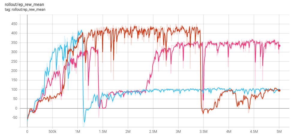
Another element that is even more annoying is the absence of good hyperparameters. At first, I used the default values, but the training suffered from catastrophic forgetting. As you can see on the graph below, the mean reward drops sharply and struggles to recover.
Rather than starting an extensive hyperparameter search, I took inspiration from the RL baselines3 Zoo configurations. After a few tweaks, I had a great set of values. Still, the policy could doubtless be further improved with hyperparameter optimization.
Exporting the Policy Network
Training a good policy is only half the work. The final objective is to submit a solution on CodinGame. Two hurdles made it non-trivial: Pytorch is not supported, and the submission must be shorter than 100k characters.
Pytorch Modules without Pytorch
Since v1.7.0, Pytorch has the fx subpackage which contains three components:
a symbolic tracer, an intermediate representation, and Python code generation.
By employing a symbolic tracing, you obtain a graph that can be transformed.
Finally, the last bit generates a valid code with match the graph’s semantic.
Unfortunately, the code generator covers only the module’s forward() method.
For the __init__(), I wrote the code generation to traverse through
all modules and print all parameter weights. Finally, since Pytorch is unavailable
in the environment, I had to implement three Pytorch modules in pure numpy:
Sequential, Linear, and ReLU.
The exported module is self-contained and combines both parameter weights and a computation graph. The result looks something like this:
import numpy as np
from numpy import float32

class MarsLanderPolicy:
    def __init__(self):
        self.policy_net = Sequential(
            Linear(
                weight=np.array([[-6.22188151e-02, -9.03800875e-02,  ...], ...], dtype=float32),
                bias=np.array([-0.03082988,  0.05894076, ...], dtype=float32),
            ),
            ReLU(),
            Linear(
                weight=np.array([[ 6.34499416e-02, -1.32812252e-02,,  ...], ...], dtype=float32),
                bias=np.array([-0.0534077 , -0.02541942, ...], dtype=float32),
            ),
            ReLU(),
        )
        self.action_net = Linear(
            weight=np.array([[-0.07862598, -0.01890517, ...], ...], dtype=float32),
            bias=np.array([0.08827707, 0.10649449], dtype=float32)),
        )

    def forward(self, observation):
        policy_net_0 = getattr(self.policy_net, "0")(observation);  observation = None
        policy_net_1 = getattr(self.policy_net, "1")(policy_net_0);  policy_net_0 = None
        policy_net_2 = getattr(self.policy_net, "2")(policy_net_1);  policy_net_1 = None
        policy_net_3 = getattr(self.policy_net, "3")(policy_net_2);  policy_net_2 = None
        action_net = self.action_net(policy_net_3);  policy_net_3 = None
        return action_net
Encoding for Shortening
As good as it looks, the exported solution is way too long at 440k characters.

The model has 71 input values, two hidden layers with 128 activations and two output nodes, which represents 25,858 free parameters. We could train a shallower network, but let’s see if we can find a way to shrink the generated code by at least 78%.
Each parameter is a 32-bit float, which takes, on average, 16 characters in plain text. Even when truncating to float16, the exported module is only ~100k chars shorter.
Clearly, printing all the floating numbers decimals is expensive. A different representation must be used! The shortest solution is obtained by taking the base64 encoding of the buffers filled with half float. The solution is now only 75k chars long.
I had one more trick up my sleeve in case base64 had been insufficient. So far, I have only been using chars contained in the ASCII table. The hack is to group two consecutive UTF-8 chars into one UTF-16 char. It’s way less readable and practical, but this yields another 50% reduction! Look at this monstrosity:
exec(bytes('浩潰瑲猠獹椊灭牯⁴慭桴䜊㴠㌠㜮ㄱ圊䑉䡔㴠㜠〰ਰ䕈䝉呈㴠㌠〰ਰ⸮ ... ⸮ਮ牰湩⡴≦牻畯摮愨杮敬紩笠潲湵⡤桴畲瑳紩⤢','u16')[2:])
With these three techniques combined (numerical approximation, buffer encoding and text encoding) it would have been possible to accommodate a model with 2.75 times more learnable parameters.
Conclusion
At the time of writing, with a cumulated 2,257 liters of fuel left, this solution puts me in 225th place over 4,986 contestants. The policy only takes between 8ms and 10ms.
This project was quite fun and a great opportunity for some hands-on RL practice. For me, the main takeaway is that RL uses the same nuts and bolts as other ML projects. Simplify the problem, always use visualization, provide good input, and don’t expect default hyperparameters to work on your task.
Have a look at the repo (MIT license) antoinebrl/rl-mars-lander if you want to play the game, use the environment or use the trained agent.